In this article we'll be trying to solve the puzzle game flood using Python. The game is played on a grid of cells that can be of any fixed number of colors. The goal is, starting with the top left cell, pick a color to switch all adjacent cells to until the entire grid has cells of the same color.
The game can be played on a variety of platforms including online thanks to Simon Tatham. Be sure to check out all the other puzzles which are equally interesting I recommend Inertia, Net and Same Game.
Preliminaries
In order to try and solve one of these puzzles, we first need to create one. We could either write our own implementation of the game (doable but a lot of extra work) or extract puzzles from Simon Tatham's version. Thankfully the code for the game is open-source so we can try the latter. A copy of the code for Simon Tatham's puzzle collection can be obtained with:
git clone https://git.tartarus.org/simon/puzzles.git
We can use the already defined dump_grid function by making some changes to
flood.c. Save the following to a file and run git apply <somefile>
diff --git a/flood.c b/flood.c
index bef45f3..938a580 100644
--- a/flood.c
+++ b/flood.c
@@ -287,7 +287,7 @@ static void free_scratch(struct solver_scratch *scratch)
     sfree(scratch);
 }

-#if
+#if 1
 /* Diagnostic routines you can uncomment if you need them */
 void dump_grid(int w, int h, const char *grid, const char *titlefmt, ...)
 {
@@ -658,6 +658,8 @@ static game_state *new_game(midend *me, const game_params *params,
     state->solnpos = 0;
     state->soln = NULL;

+    printf("%d by %d with %d -> %d\n", state->w, state->h, params->leniency ,state->movelimit);
+    dump_grid(w, h, state->grid, "");
     return state;
 }
After the change, we can compile the game following the instructions in the
project's README. To collect the data we want, we run the game while
redirecting the output to a file i.e. ./flood > easy.txt. A new puzzle is
produced and written to this file when the program starts and each time we
start a new game.
Loading A Puzzle
I produced a few puzzles of varying difficulty and grid size using the method above. In order to load the puzzles into our program, we need to parse text structured as follows.
12 by 12 -> 23
  220512241115
  050301010135
  145334435442
  055410020501
  115015101341
  540123454434
  005154123544
  342420355535
  412520311103
  554304552042
  255022011245
  212510012340
The first line represents the dimensions of the board (12 wide and 12 tall) and the maximum number of moves needed to solve the puzzle (23). The lines that follow correspond to the actual board. Each individual number represents a cell in the grid with the value corresponding to a particular color.
Given the nature of flood, the most obvious way to represent the
board is with a 2D list. Each row corresponding to a list and each column an
entry within the list. The first row for the above puzzle would be
[2, 2, 0, 5, 1, 2, 2, 4, 1, 1, 1, 5].
However, since in order to solve the puzzle we need to mutate the state of the board frequently using a list would necessitate copying every time we pass the board to a function. The reason for this is that lists in Python are passed by reference and not by value.
a = [1, 2, 3, 4, 5]
def f(some_list):
    some_list[0] = 6
    return some_list

f(a)        # => [6, 2, 3, 4, 5]
a == f(a)   # => True
Instead of using a list, we instead implement a simple Grid data structure to hold the board.
class Grid:
    def __init__(self, grid):
        self._grid = tuple(tuple(row) for row in grid)
        self._rows = len(grid)
        self._cols = len(grid[0]) if grid else 0

    def __getitem__(self, index):
        row, col = index
        return self._grid[row][col]

    def __setitem__(self, row, col, value):
        new_grid = [list(row) for row in self._grid]
        new_grid[row][col] = value
        return Grid(new_grid)

    def __iter__(self):
        """Iterator over grid positions."""
        for i in range(self._rows):
            for j in range(self._cols):
                yield (i, j)

    def __repr__(self):
        return f"Grid({[list(row) for row in self._grid]})"

    # necessary for using Grid as a dict key
    def __hash__(self):
        return hash(tuple(self[i, j] for (i, j) in iter(self)) + (self.rows, self.cols))

    # looks odd but we'll see why it's necessary later
    def __lt__(self, other):
        return False

    @property
    def rows(self):
        return self._rows

    @property
    def cols(self):
        return self._cols

    def set_mul(self, positions, value):
        """Change multiple grid positions."""
        new_grid = [list(row) for row in self._grid]
        for row, col in positions:
            new_grid[row][col] = value
        return Grid(new_grid)

    def is_valid(self, pos):
        """Check if position is on grid."""
        row, col = pos
        return (0 <= row < self._rows) and (0 <= col < self._cols)
When parsing the puzzle, other than the board itself we also keep track of the dimensions of the puzzles (although this can be inferred by the shape of the grid), and the maximum amount of moves needed to solve the puzzle.
import re

easy = "puzzles/easy_5.txt"
medi = "puzzles/medium_5.txt"
hard = "puzzles/hard_5.txt"


def parse_header(header):
    p = re.compile(r"(?P<width>\d{1,2}) by (?P<height>\d{1,2}) -> (?P<mmoves>\d{1,2})")
    if m := re.match(p, header):
        return {k: int(v) for k, v in m.groupdict().items()}


def parse_puzzles(file):
    puzzles = []
    with open(file, "r") as fp:
        while line := fp.readline():
            if line.strip():
                meta = parse_header(line.strip())
                board = []
                for _ in range(meta["height"]):
                    r = list(map(int, iter(fp.readline().strip())))
                    board.append(r)
                puzzles.append(meta | {"board": Grid(board)})
    return puzzles


peasy = parse_puzzles(easy)
pmedi = parse_puzzles(medi)
phard = parse_puzzles(hard)

peb0 = peasy[0]["board"]
The final preliminary step we need to complete is displaying the board, since the original puzzle has a graphical form we'll replicate it. We also add the ability to highlight specific cells within the grid with a white border.
from PIL import Image, ImageDraw, ImageFont

color_map = ["red", "yellow", "green", "blue", "orange", "purple"]


def show_puzzle(board, highlight=None, cell_width=40, debug=False):
    width = board.cols
    height = board.rows
    image = Image.new("RGB", (cell_width * width, cell_width * height), (0, 0, 0))
    draw = ImageDraw.Draw(image)
    fnt = ImageFont.truetype("/usr/share/fonts/TTF/FiraCode-Bold.ttf", size=16)
    y0 = 0
    y1 = cell_width
    x0 = 0
    x1 = cell_width
    for i, j in board:
        x0 = cell_width * j
        y0 = cell_width * i
        x1 = cell_width * (j + 1)
        y1 = cell_width * (i + 1)
        if highlight is not None and (i, j) in highlight:
            draw.rectangle(
                [x0, y0, x1, y1],
                fill=color_map[board[i, j]],
                outline="white",
                width=4,
            )
        else:
            draw.rectangle(
                [x0, y0, x1, y1],
                fill=color_map[board[i, j]],
                outline="black",
                width=2,
            )
        if debug:
            draw.text(
                (x0 + cell_width // 2, y0 + cell_width // 2),
                f"{i}, {j}",
                anchor="mm",
                fill=(0, 0, 0, 255),
            )
    return image
We can view one of our loaded puzzles by using .show() or .save(file) on
the image returned by show_puzzle e.g show_puzzle(peb0).show()

Simulating Moves
Since we can now visualize the board, we need to be able to change the state of the board i.e. play the game. You can see an example of how the game is played below:
In order to simulate the rules of the game we need to be able to do the following:
- Find cells neighbouring a particular position.
- Find all cells connected to a position by color i.e. a cluster.
- Find cells neighbouring a cluster.
The first step involves some simple math with a check (Board.is_valid)
to make sure the positions are within our board grid. We use a set to ensure
that no positions are repeated and to also make testing for the presence
of a particular position fast and easy.
def find_neighbours(position, board):
    neighbourhood = [
        (0, -1),
        (-1, 0),
        (+1, 0),
        (0, +1),
    ]
    return set(
        filter(
            lambda x: board.is_valid(x),
            [(i[0] + position[0], i[1] + position[1]) for i in neighbourhood],
        )
    )
Finding the cluster containing a position is a little more involved. We start with said position as the only member of the cluster and extending with that position's neighbours with the same color. This is repeated for each of the neighbours that are added to the cluster. We use a set for the same reasons as above.
def find_cluster_containing(position, board):
    cluster = {position}
    color_matches = lambda p: board[p] == board[position]
    neighbours = find_neighbours(position, board)
    while neighbours:
        n = neighbours.pop()
        if color_matches(n):
            cluster.add(n)
            neighbours |= find_neighbours(n, board) - cluster
    return cluster
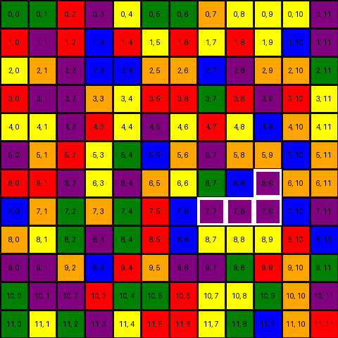
We can try out the function by finding and highlighting the cluster containing the position
(7, 9) with show_puzzle(peb0, debug=True, highlight=find_cluster_containing((7, 9), peb0)).show()
One more additional function that might be useful is being able to find the
neighbours of a cluster. We can do this by finding the neighbours of each
member, filtering any duplicates and combining them into a single set. We use
some FP to make this easy but find_cluster_neighbours2 shows the equivalent
imperative version.
from functools import partial, reduce
from operator import or_
def find_cluster_neighbours(cluster, board):
return (
set(reduce(or_, map(partial(find_neighbours, board=board), cluster))) - cluster
)
def find_cluster_neighbours2(cluster, board):
res = set()
for i in cluster:
res |= find_neighbours(i, board)
return res - cluster
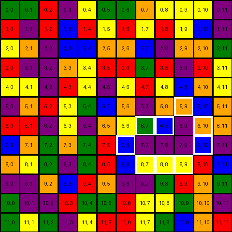
c1 = find_cluster_containing((7, 9), peb0)
i1 = show_puzzle(peb0, debug=True, highlight=find_cluster_neighbours(c1, peb0))
With all these functions defined we can finally implement one to make a move.
A move is made by looking for the cluster containing the cell (0, 0) then
changing it's color to a new one, which effectively extends the cluster.
def move(color, board):
    main_cluster = find_cluster_containing((0, 0), board)
    color = color_map.index(color) if isinstance(color, str) else color
    cluster_neighbours = set()
    for i in main_cluster:
        cluster_neighbours |= find_neighbours(i, board)
    if any([board[i] == color for i in cluster_neighbours]):
        return board.set_mul(main_cluster, color)
    return board


peb00 = move("red", peb0)
i2 = show_puzzle(peb00)

To create a way to 'play' the game we use a simple loop that
shows the board, reads user input and calls move until the
board is solved.
def find_color(c):
    return next(i for i in color_map if i[0] == c)


def play(board):
    while not is_solved(board):
        i = show_puzzle(board)
        i.show()
        choices = [i[0] for i in color_map]
        color = input(f"pick a color {' '.join(choices)}> ")
        if color in choices:
            board = move(board, find_color(color))
        else:
            return board
    return
Writing A Solver
The easiest method to solve a problem of this nature would be the brute-force approach. We'd generate every single move possible for a particular puzzle and pick the sequence of moves that lead to a solution the fastest. Sound pretty simple.
The downside of this approach and the reason it's not used much in practice is that enumerating every possibility may be impossible, take too much time, or use too much memory. The advantage of this approach is that by enumerating and exploring all possible options, we can guarantee finding an optimal solution if one exists.
An optimal solution refers to a solution that is the best according to a specific criteria. In our case the optimal solution would be the one with the smallest series of color changes that transforms the entire grid into a singular color.
Finding a solution involves looking through the different states of the problem resulting from a particular action. In our case we're looking through the states of the board after a move is made. These states are commonly referred to as the search space and can be thought of as a graph where the nodes are individual states and the edges represent actions that transition from one state to another.
The specific way we choose to look through the search space is what distinguishes different algorithms i.e Depth-First Search or Breadth-First Search. As you may have already guessed from the title we use the A* algorithm to limit how much of the search space we look through while still being able to find a reasonable solution.
The A* Algorithm
If we look at the description from the WikiPedia page:
A* is an informed search algorithm, or a best-first search, meaning that it is formulated in terms of weighted graphs: starting from a specific starting node of a graph, it aims to find a path to the given goal node having the smallest cost (least distance travelled, shortest time, etc.). It does this by maintaining a tree of paths originating at the start node and extending those paths one edge at a time until the goal node is reached.
Calculating the cost of each path is where A* differs from something like Dijkstra's algorithm. Specifically it picks a path while taking into account an additional value from a heuristic. This extra consideration minimizes how much of the search space we need to explore to find a solution.
Implementation
We'll jump right into the code before explaining what each part does.
import heapq
from icecream import ic


def find_all_clusters(board):
    positions = set(iter(board))
    while positions:
        pos = positions.pop()
        c = find_cluster_containing(pos, board)
        positions -= c
        yield c


# the heuristic function
def cluster_count(board):
    main = find_cluster_containing((0, 0), board)
    count = 0
    for c in find_all_clusters(board):
        if c == main:
            continue
        count += 1
    return count


def a_star_solve(initial_board, heuristic=cluster_count):
    open_set = []
    heapq.heappush(open_set, (0, initial_board))
    came_from = {}
    g_score = {initial_board: 0}
    f_score = {initial_board: heuristic(initial_board)}

    while open_set:
        current = heapq.heappop(open_set)[1]

        if is_solved(current):
            return reconstruct_path(came_from, current)

        cluster = find_cluster_containing((0, 0), current)
        # valid moves
        maybe_colors = {current[x] for x in find_cluster_neighbours(cluster, current)}
        for next_board in [move(c, current) for c in maybe_colors]:
            tentative_g_score = g_score[current] + 1
            if next_board not in g_score or tentative_g_score < g_score[next_board]:
                came_from[next_board] = current
                g_score[next_board] = tentative_g_score
                f_score[next_board] = tentative_g_score + heuristic(next_board)
                e = (f_score[next_board], next_board)
                if e not in open_set:
                    heapq.heappush(open_set, e)
    return None


def reconstruct_path(came_from, current):
    cluster = find_cluster_containing((0, 0), current)
    color = current[cluster.pop()]
    total_path = [color]
    while current in came_from.keys():
        current = came_from[current]
        cluster = find_cluster_containing((0, 0), current)
        color = current[cluster.pop()]
        total_path.append(color)
    return total_path[::-1][1:]


def is_solved(board):
    return len(set(board[i, j] for (i, j) in board)) == 1
Before going over the details let's try and run the solver. We save the result in a GIF to make it easier to inspect.
sol = a_star_solve(peb0)    # [2, 0, 5, 0, 1, 4, 5, 2, 0, 4, 1, 3, 5, 2, 0, 1, 4, 3, 5, 0, 2, 3]
b = peb0


def show_solution(sol, board, outfile="solve.gif"):
    imgs = []
    b = board
    for c in sol:
        b = move(c, b)
        imgs.append(show_puzzle(b))
    imgs[0].save(
        outfile, save_all=True, append_images=imgs[1:], optimize=False, duration=500
    )


show_solution(sol, peb0, "easy-1-solve.gif")
Explanation, Evaluation and Improvement
From the GIF above we can see that our implementation does indeed find a
viable solution for the flood puzzle. We can further verify this by making
sure that the returned solution is shorter than the maximum moves expected.
(len(sol) <= peasy[0]['mmoves']).
Our implementation matches pretty closely with the pseudocode in the WikiPedia page. Some important things to keep in mind are:
- The heuristic function can be changed to improve the performance of the whole algorithm. In our case we count the number of unique clusters remaining on the board.
heapqis used for the priority queue. We added__lt__toGridearlier to simplify usage ofheapqwhich does comparison with<. The way__lt__is implemented means that selecting an item from the queue is based entirely on the f-score of the board. This shouldn't make a difference but I may be missing something.
We can try and graph how our heuristic performs across the different puzzle difficulties. To do that we'll first produce the data then plot a graph using the vega-lite online editor.
def generate_data(puzzles, difficulty="easy"):
    data = []
    for i, p in enumerate(puzzles):
        data.extend(
            [
                {
                    "difficulty": difficulty,
                    "type": "expected",
                    "value": p["mmoves"],
                    "index": i,
                },
                {
                    "difficulty": difficulty,
                    "type": "actual",
                    "value": len(a_star_solve(p["board"])),
                    "index": i,
                },
            ]
        )
    return data


data = (
    generate_data(peasy, "easy")
    + generate_data(pmedi, "medium")
    + generate_data(phard, "hard")
)
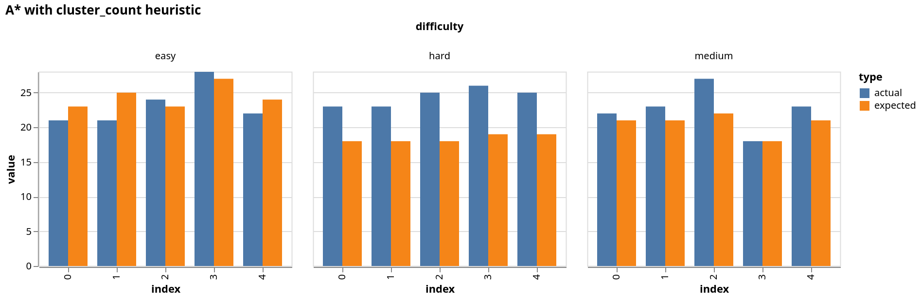
As we can see our heuristic doesn't really perform as well as we'd hope. The
good news is that we can use a different heuristic. I tried a couple different
ones such as evaluating the size of the main cluster but none that matched
the performance of cluster_count. From what I saw Simon Tatham uses
backtracking search which works very well. I believe a heuristic that uses
some form of lookahead would perform similarly. I'll leave that as an exercise
for the reader (😆). Anyone with some other interesting heuristics can leave
a comment below.
I hope you found this article illuminating, I'll catch you in the next one.
Final Thoughts
- I used Literate Programming to write the code and text for this article through Quarto. I write Quarto markdown in neovim with the plugins quarto-nvim and vim-slime. The former allows syntax highlighting and language server support in code blocks within markdown and the latter lets you run code from your editor in a separate REPL.
- I'll be exploring how to solve some of the other puzzles in Simon Tatham's collection using different of approaches. Stay tuned for more.
- The repo for this project can be found on GitHub